6 Summarise

6.1 Learning Objectives

Use summary functions to explore the structure and completeness of a dataset.
Create simple summaries and grouped summaries using count(), group_by(), and summarise().
Calculate descriptive statistics (mean, SD) across groups.
Use janitor tools Firke (2024) to quickly tabulate and summarise categorical data.

6.2 A first glimpse

When starting with a new dataset, we want to get an initial idea:

How many rows and columns are there?
What are the column names?
What types of data are in each column?
What are their possible values or ranges?
These answers are useful to know before jumping into wrangling and cleaning data.

There are several ways to return an overview of your data, ranging in how comprehensively you wish to summarise your data’s structure.

glimpse(penguins_raw)

Rows: 344
Columns: 17
$ studyName             <chr> "PAL0708", "PAL0708", "PAL0708", "PAL0708", "PAL…
$ `Sample Number`       <dbl> 1, 2, 3, 4, 5, 6, 7, 8, 9, 10, 11, 12, 13, 14, 1…
$ Species               <chr> "Adelie Penguin (Pygoscelis adeliae)", "Adelie P…
$ Region                <chr> "Anvers", "Anvers", "Anvers", "Anvers", "Anvers"…
$ Island                <chr> "Torgersen", "Torgersen", "Torgersen", "Torgerse…
$ Stage                 <chr> "Adult, 1 Egg Stage", "Adult, 1 Egg Stage", "Adu…
$ `Individual ID`       <chr> "N1A1", "N1A2", "N2A1", "N2A2", "N3A1", "N3A2", …
$ `Clutch Completion`   <chr> "Yes", "Yes", "Yes", "Yes", "Yes", "Yes", "No", …
$ `Date Egg`            <chr> "11/11/2007", "11/11/2007", "16/11/2007", "16/11…
$ `Culmen Length (mm)`  <dbl> 39.1, 39.5, 40.3, NA, 36.7, 39.3, 38.9, 39.2, 34…
$ `Culmen Depth (mm)`   <dbl> 18.7, 17.4, 18.0, NA, 19.3, 20.6, 17.8, 19.6, 18…
$ `Flipper Length (mm)` <dbl> 181, 186, 195, NA, 193, 190, 181, 195, 193, 190,…
$ `Body Mass (g)`       <dbl> 3750, 3800, 3250, NA, 3450, 3650, 3625, 4675, 34…
$ Sex                   <chr> "MALE", "FEMALE", "FEMALE", NA, "FEMALE", "MALE"…
$ `Delta 15 N (o/oo)`   <dbl> NA, 8.94956, 8.36821, NA, 8.76651, 8.66496, 9.18…
$ `Delta 13 C (o/oo)`   <dbl> NA, -24.69454, -25.33302, NA, -25.32426, -25.298…
$ Comments              <chr> "Not enough blood for isotopes.", NA, NA, "Adult…

str(penguins_raw)

spc_tbl_ [344 × 17] (S3: spec_tbl_df/tbl_df/tbl/data.frame)
 $ studyName          : chr [1:344] "PAL0708" "PAL0708" "PAL0708" "PAL0708" ...
 $ Sample Number      : num [1:344] 1 2 3 4 5 6 7 8 9 10 ...
 $ Species            : chr [1:344] "Adelie Penguin (Pygoscelis adeliae)" "Adelie Penguin (Pygoscelis adeliae)" "Adelie Penguin (Pygoscelis adeliae)" "Adelie Penguin (Pygoscelis adeliae)" ...
 $ Region             : chr [1:344] "Anvers" "Anvers" "Anvers" "Anvers" ...
 $ Island             : chr [1:344] "Torgersen" "Torgersen" "Torgersen" "Torgersen" ...
 $ Stage              : chr [1:344] "Adult, 1 Egg Stage" "Adult, 1 Egg Stage" "Adult, 1 Egg Stage" "Adult, 1 Egg Stage" ...
 $ Individual ID      : chr [1:344] "N1A1" "N1A2" "N2A1" "N2A2" ...
 $ Clutch Completion  : chr [1:344] "Yes" "Yes" "Yes" "Yes" ...
 $ Date Egg           : chr [1:344] "11/11/2007" "11/11/2007" "16/11/2007" "16/11/2007" ...
 $ Culmen Length (mm) : num [1:344] 39.1 39.5 40.3 NA 36.7 39.3 38.9 39.2 34.1 42 ...
 $ Culmen Depth (mm)  : num [1:344] 18.7 17.4 18 NA 19.3 20.6 17.8 19.6 18.1 20.2 ...
 $ Flipper Length (mm): num [1:344] 181 186 195 NA 193 190 181 195 193 190 ...
 $ Body Mass (g)      : num [1:344] 3750 3800 3250 NA 3450 ...
 $ Sex                : chr [1:344] "MALE" "FEMALE" "FEMALE" NA ...
 $ Delta 15 N (o/oo)  : num [1:344] NA 8.95 8.37 NA 8.77 ...
 $ Delta 13 C (o/oo)  : num [1:344] NA -24.7 -25.3 NA -25.3 ...
 $ Comments           : chr [1:344] "Not enough blood for isotopes." NA NA "Adult not sampled." ...
 - attr(*, "spec")=
  .. cols(
  ..   studyName = col_character(),
  ..   `Sample Number` = col_double(),
  ..   Species = col_character(),
  ..   Region = col_character(),
  ..   Island = col_character(),
  ..   Stage = col_character(),
  ..   `Individual ID` = col_character(),
  ..   `Clutch Completion` = col_character(),
  ..   `Date Egg` = col_character(),
  ..   `Culmen Length (mm)` = col_double(),
  ..   `Culmen Depth (mm)` = col_double(),
  ..   `Flipper Length (mm)` = col_double(),
  ..   `Body Mass (g)` = col_double(),
  ..   Sex = col_character(),
  ..   `Delta 15 N (o/oo)` = col_double(),
  ..   `Delta 13 C (o/oo)` = col_double(),
  ..   Comments = col_character()
  .. )
 - attr(*, "problems")=<externalptr>

library(skimr)

skim(penguins_raw)

Data summary
Name	penguins_raw
Number of rows	344
Number of columns	17
_______________________
Column type frequency:
character	10
numeric	7
________________________
Group variables	None

Variable type: character

skim_variable	n_missing	complete_rate	min	max	n_unique
studyName	0	1.00	7	7	3
Species	0	1.00	33	41	3
Region	0	1.00	6	6	1
Island	0	1.00	5	9	3
Stage	0	1.00	18	18	1
Individual ID	0	1.00	4	6	190
Clutch Completion	0	1.00	2	3	2
Date Egg	0	1.00	10	10	50
Sex	11	0.97	4	6	2
Comments	290	0.16	18	68	10

Variable type: numeric

skim_variable	n_missing	complete_rate	mean	sd	p0	p25	p50	p75	p100	hist
Sample Number	0	1.00	63.15	40.43	1.00	29.00	58.00	95.25	152.00	▇▇▆▅▃
Culmen Length (mm)	2	0.99	43.92	5.46	32.10	39.23	44.45	48.50	59.60	▃▇▇▆▁
Culmen Depth (mm)	2	0.99	17.15	1.97	13.10	15.60	17.30	18.70	21.50	▅▅▇▇▂
Flipper Length (mm)	2	0.99	200.92	14.06	172.00	190.00	197.00	213.00	231.00	▂▇▃▅▂
Body Mass (g)	2	0.99	4201.75	801.95	2700.00	3550.00	4050.00	4750.00	6300.00	▃▇▆▃▂
Delta 15 N (o/oo)	14	0.96	8.73	0.55	7.63	8.30	8.65	9.17	10.03	▃▇▆▅▂
Delta 13 C (o/oo)	13	0.96	-25.69	0.79	-27.02	-26.32	-25.83	-25.06	-23.79	▆▇▅▅▂

At this early stage, it’s helpful to assess whether your dataset meets your expectations. Consider if the data appear as anticipated. Are the values in each column reasonable? Are there any noticeable gaps or errors that might need to be corrected, or that could potentially render the data unusable?

Your turn

The dataset has rows (including the headers) and 17 columns.

It also provides information on the type of data in each column

<chr> - means character or text data
<dbl> - means numerical data

Q Based on our summary functions are any variables assigned to the wrong data type (should be character when numeric or vice versa)?

Although some columns like date might not be correctly treated as character variables, they are not strictly numeric either, all other columns appear correct

Q Based on our summary functions do we have complete data for all variables?

No, they are 2 missing data points for body measurements (culmen, flipper, body mass), 11 missing data points for sex, 13/14 missing data points for blood isotopes (Delta N/C) and 290 missing data points for comments

We have just learned some ways to initially inspect our dataset. Keep in mind, we don’t expect everything to be perfect. This initial inspection is a good opportunity to identify where these issues might be and assess their severity.

When you are confident that the dataset is largely as expected, you are ready to start summarising your data.

6.3 Summary counts

In the previous section, we learned how to get an overview of our data’s structure, including the number of rows, the columns present, and any missing data. In this section, we will focus on summarising the data. Summarising data can provide insight into the scope and variation in our dataset, and help in evaluating its suitability for our analysis.

With our data we can count the total number of occurrences for different groups either by:

6.3.1 Filtering

penguins_raw |> 
  filter(`Species` == "Adelie Penguin (Pygoscelis adeliae)") |> 
  count()

n
152

6.3.2 Grouping

Or by grouping :

penguins_raw |> 
  group_by(Species) |> 
  count()

Species	n
Adelie Penguin (Pygoscelis adeliae)	152
Chinstrap penguin (Pygoscelis antarctica)	68
Gentoo penguin (Pygoscelis papua)	124

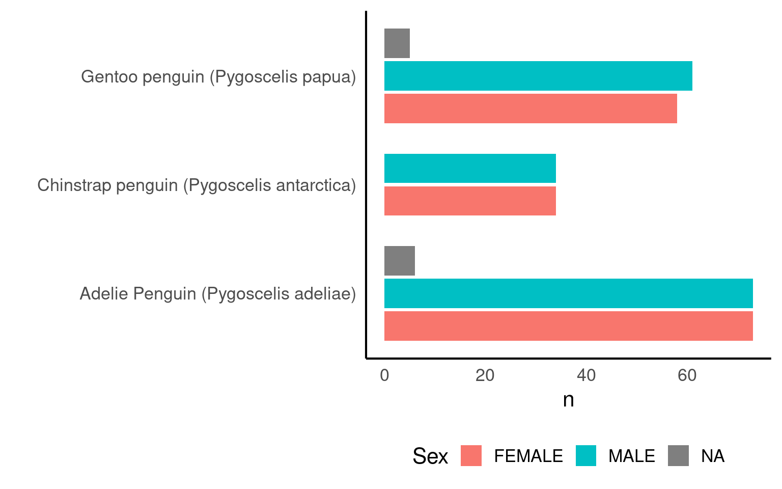
6.4 Frequency counts by subgroups

We can apply multiple grouping parameters at the same time - for example if we wish to know the frequency of observations by species and sex.

We can do this using dplyr or with functions in the janitor package:

penguins_raw |> 
  group_by(Species,Sex) |> 
  count() |> 
  arrange(desc(n))

Species	Sex	n
Adelie Penguin (Pygoscelis adeliae)	FEMALE	73
Adelie Penguin (Pygoscelis adeliae)	MALE	73
Gentoo penguin (Pygoscelis papua)	MALE	61
Gentoo penguin (Pygoscelis papua)	FEMALE	58
Chinstrap penguin (Pygoscelis antarctica)	FEMALE	34
Chinstrap penguin (Pygoscelis antarctica)	MALE	34
Adelie Penguin (Pygoscelis adeliae)	NA	6
Gentoo penguin (Pygoscelis papua)	NA	5

penguins_raw |>
  tabyl(Sex, Species) |> 
  adorn_percentages("all") |>
  adorn_totals(c("row", "col")) |>
  adorn_pct_formatting(digits = 1)

Sex	Adelie Penguin (Pygoscelis adeliae)	Chinstrap penguin (Pygoscelis antarctica)	Gentoo penguin (Pygoscelis papua)	Total
FEMALE	21.2%	9.9%	16.9%	48.0%
MALE	21.2%	9.9%	17.7%	48.8%
NA	1.7%	0.0%	1.5%	3.2%
Total	44.2%	19.8%	36.0%	100.0%

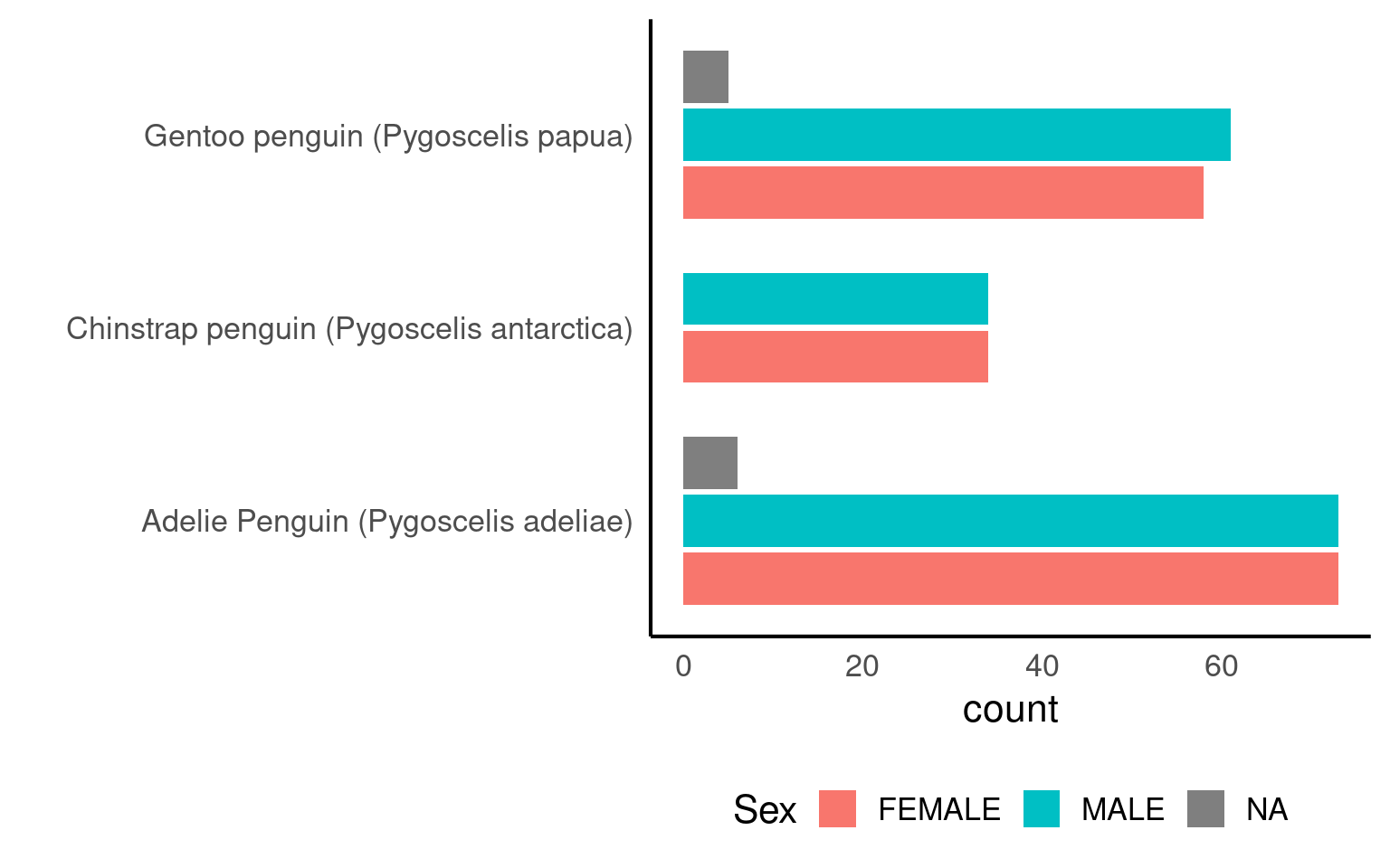
6.5 Visualising Frequencies

Graphs make summaries easier to interpret at a glance.

penguins_raw |> 
  group_by(Species,Sex) |> 
  count() |> 
  arrange(desc(n)) |> 
  ggplot(aes(x = Species,
             y = n,
             fill = Sex))+
  geom_col(position=position_dodge2(preserve="single"))+
  coord_flip()+
  labs(x = "")+
  theme(legend.position = "bottom")

penguins_raw |> 
  ggplot(aes(x = Species,
             fill = Sex))+
  geom_bar(position=position_dodge2(preserve="single"))+
  coord_flip()+
  labs(x = "")+
  theme(legend.position = "bottom")

6.6 Summary statistics

We can extend our summaries to show not just counts, but also measures of central tendency (mean) and spread (standard deviation).

These are powerful ways to understand variation within groups.

penguins_raw |>
group_by(Species) |> # Calculate withing groups
summarise(
mean_mass = mean(`Body Mass (g)`, na.rm = TRUE),
sd_mass = sd(`Body Mass (g)`, na.rm = TRUE),
n = n()
)

Species	mean_mass	sd_mass	n
Adelie Penguin (Pygoscelis adeliae)	3700.662	458.5661	152
Chinstrap penguin (Pygoscelis antarctica)	3733.088	384.3351	68
Gentoo penguin (Pygoscelis papua)	5076.016	504.1162	124

Your turn

Add Sex to the group_by() function to see how mean and SD of body mass differ by sex within species.

penguins_raw |>
group_by(Species, Sex) |> 
drop_na(Sex) |> # Optional remove rows where Sex is unknown
summarise(
mean_mass_g = mean(`Body Mass (g)`, na.rm = TRUE),
sd_mass_g = sd(`Body Mass (g)`, na.rm = TRUE),
n = n()
)

Species	Sex	mean_mass_g	sd_mass_g	n
Adelie Penguin (Pygoscelis adeliae)	FEMALE	3368.836	269.3801	73
Adelie Penguin (Pygoscelis adeliae)	MALE	4043.493	346.8116	73
Chinstrap penguin (Pygoscelis antarctica)	FEMALE	3527.206	285.3339	34
Chinstrap penguin (Pygoscelis antarctica)	MALE	3938.971	362.1376	34
Gentoo penguin (Pygoscelis papua)	FEMALE	4679.741	281.5783	58
Gentoo penguin (Pygoscelis papua)	MALE	5484.836	313.1586	61

6.6.1 Summarise multiple variables

summarise_at()

Summarise specific selected variables:

penguins_raw |> 
  group_by(Species) |> 
  summarise_at(c("Flipper Length (mm)", "Culmen Length (mm)", "Culmen Depth (mm)"),
               mean,
               na.rm =T)

Species	Flipper Length (mm)	Culmen Length (mm)	Culmen Depth (mm)
Adelie Penguin (Pygoscelis adeliae)	189.9536	38.79139	18.34636
Chinstrap penguin (Pygoscelis antarctica)	195.8235	48.83382	18.42059
Gentoo penguin (Pygoscelis papua)	217.1870	47.50488	14.98211

summarise_if()

penguins_raw |> 
  group_by(Species) |> 
  summarise_if(is.numeric, mean, na.rm =T)

Species	Sample Number	Culmen Length (mm)	Culmen Depth (mm)	Flipper Length (mm)	Body Mass (g)	Delta 15 N (o/oo)	Delta 13 C (o/oo)
Adelie Penguin (Pygoscelis adeliae)	76.5	38.79139	18.34636	189.9536	3700.662	8.859733	-25.80419
Chinstrap penguin (Pygoscelis antarctica)	34.5	48.83382	18.42059	195.8235	3733.088	9.356155	-24.54654
Gentoo penguin (Pygoscelis papua)	62.5	47.50488	14.98211	217.1870	5076.016	8.245338	-26.18530

6.6.2 Useful `summary` functions

6.6.2.1 Measure of location:

mean(x): sum of x divided by the length
median(x): 50% of x is above and 50% is below

6.6.2.2 Measure of variation:

sd(x): standard deviation
IQR(x): interquartile range (robust equivalent of sd when outliers are present in the data)

6.6.2.3 Measure of rank:

min(x): minimum value of x
max(x): maximum value of x
quantile(x, 0.25): 25% of x is below this value

6.6.2.4 Counts:

n(x): the number of element in x
sum(!is.na(x)): count non-missing values
n_distinct(x): count the number of unique value

6.7 Summary

In this section we learned to:

Inspect structure and completeness
- Use glimpse(), str(), and skim() to understand column types, missing data, and variable ranges.
- Confirm that variables are stored in appropriate formats (e.g. numeric vs character).
Summarise counts and categories

Count observations using count() and group_by() to explore dataset composition.

Use janitor::tabyl() for fast, readable cross-tabulations and percentages.
Calculate descriptive statistics
- Compute group-wise summaries with summarise() such as means, SDs, and counts.