brand_colours <- c(
  "teal"    = "#09baba",  # bright teal
  "green"   = "#0d8242",  # dark green
  "lime"    = "#0ee565",  # vivid lime
  "navy"    = "#2c4977",  # deep navy
  "blue"    = "#3293BD",  # bright blue
  "yellow"  = "#d2db2e"   # lime-yellow accent
)

mono_palette <- function(base_col = "#2c4977", n = 5) {
  colorRampPalette(c(base_col, "white"))(n)
}

# Example use
mono_blue <- mono_palette( "#2c4977", n = 5)


brand_palettes <- list(
  brand_colours = brand_colours,
  discrete = c("#09baba", "#0d8242", "#3293BD", "#d2db2e", "#2c4977"),
  continuous_light = c("#2c4977","#09baba",  "#d2db2e" ),
  continuous_cool  = c("#09baba", "#3293BD", "#2c4977"),
  diverging        = c("#0d8242", "#d2db2e", "#3293BD"),
  mono_blue = mono_blue
)

show_brand_palettes <- function(palettes = brand_palettes) {
    df <- purrr::imap_dfr(palettes, ~{
        tibble(
            palette = .y,
            color = .x,
            order = seq_along(.x)
        )
    })

   plot <-  ggplot(df, aes(x = order, y = palette, fill = color)) +
        geom_tile(color = "white", linewidth = 0.8) +
        geom_text(aes(label = color), color = "black", size = 3, vjust = 2) +
        scale_fill_identity() +
        theme_minimal(base_size = 12) +
        theme(
            axis.title = element_blank(),
            axis.ticks = element_blank(),
            panel.grid = element_blank(),
            axis.text.x = element_blank(),
            axis.text.y = element_text(face = "bold")
        )
   plot
}19 Themes
19.1 Learning Objectives
By the end of this workshop, you will be able to:
- Apply custom themes that fit with brand design choices
In professional settings, visual outputs should communicate not only data but identity. This session shows how to translate a set of visual branding principles (colours, typography, tone) into a coherent ggplot2 theme and apply it consistently across plot types.
19.2 Making a custom palette
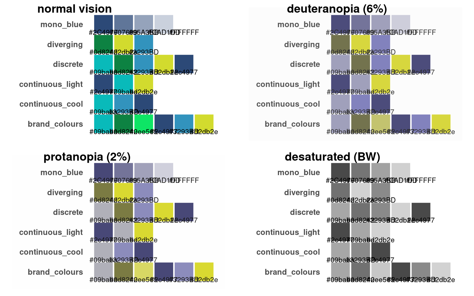
Establishing a coherent colour palette ensures every figure feels unified.
The first code block defines a named vector of brand colours, assigning meaningful names (teal, navy, yellow, etc.) to specific hex codes.
This allows the colours to be referenced consistently across plots:
19.2.1 Design check:
Which colours carry the brand’s main tone?
Which are suitable for accents or backgrounds?
Which combinations maintain legibility and contrast?

19.3 Using showtext
In R, system fonts can vary across computers — meaning your carefully chosen typography might not appear the same for others or when exporting plots. The showtext package solves this by rendering text using font files directly, ensuring consistent appearance across systems and outputs (e.g. PNG, PDF).
The simplest way to activate it is with showtext::showtext_auto() — once turned on, it applies automatically to all your plots. Check out (https://fonts.google.com/) for available fonts
library(showtext)

# Register and activate a Google font
font_add_google("Monsieur La Doulaise", "Mon")

showtext_auto()

# Use the font in ggplot
ggplot(penguins,
       aes(x = culmen_length_mm,
           y = body_mass_g,
           fill = species,
           shape = species))+
    geom_point()+
  ggtitle("A Fancy Scatterplot of Culmen length against Body Mass")+
  theme_bw(base_family ="Mon",
           base_size = 30)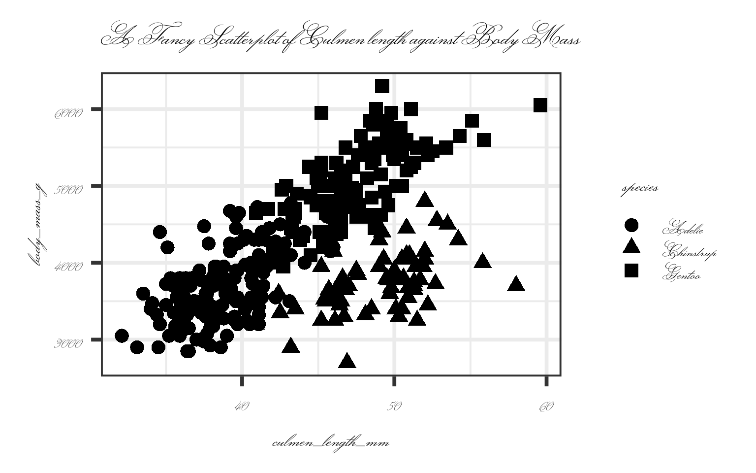
showtext_auto() makes font rendering automatic and portable — ensuring that your branded typeface appears consistently across systems, exports, and collaborators’ machines.
19.4 Construct a base theme
theme_brand <- function(base_size = 14, base_family = "Open Sans") {
  theme_minimal(base_size = base_size, base_family = base_family) +
    theme(
      # Text
      text = element_text(colour = mono_blue[1]),
      plot.title = element_text(face = "bold", size = rel(1.4), colour = mono_blue[1]),
      plot.subtitle = element_text(colour = mono_blue[2], size = rel(1.1)),
      plot.caption = element_text(size = rel(0.8), colour = mono_blue[2]),
      axis.title = element_text(face = "bold", colour = mono_blue[2]),
      axis.text = element_text(colour = mono_blue[3]),

      # Panels and gridlines
      panel.grid.major = element_line(colour = "grey90"),
      panel.grid.minor = element_blank(),
      panel.background = element_rect(fill = "white", colour = NA),

      # Facets
      strip.background = element_rect(fill = brand_colours["teal"], colour = NA),
      strip.text = element_text(face = "bold", colour = "white"),

      # Legends
      legend.title = element_text(face = "bold"),
      legend.position = "right"
    )
}
Which aspects make this “on-brand”?
Is the hierarchy of colour, text, and space clear?
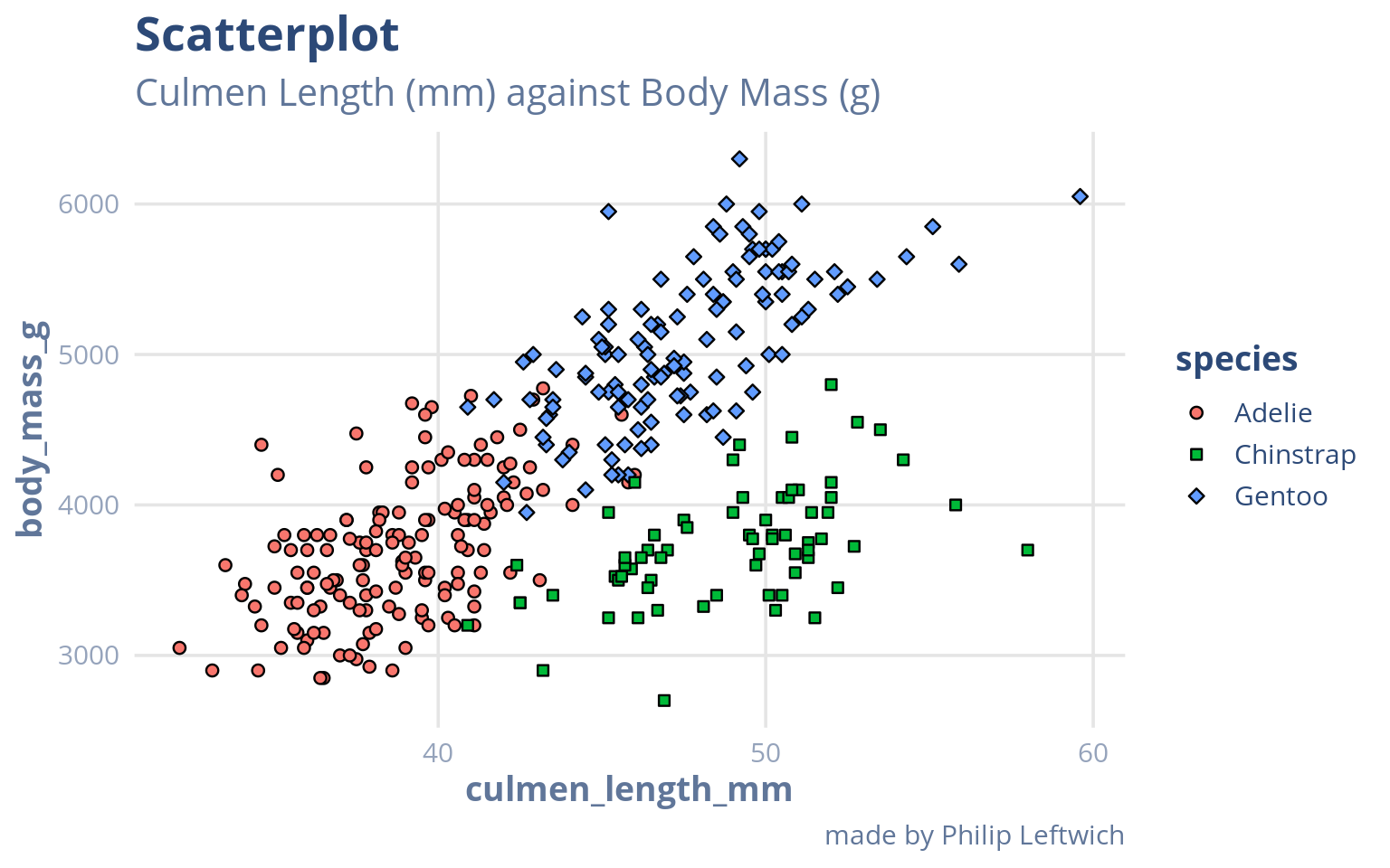
19.5 Making an advanced custom theme
A theme function defines the non-data aspects of a plot: typography, line styles, gridlines, and overall layout.
Here - theme_brand() creates a cohesive institutional style aligned with the brand colours.
Key elements to note:
Typography – the function attempts to load the Google font Open Sans via the
showtextpackage Qiu & See file AUTHORS for details. (2024), ensuring reproducible fonts across systems.Axis options – axis_type toggles between continuous and categorical grid settings, adjusting gridlines and spacing accordingly.
Colour palettes – palette selects one of the brand palette variants and attaches appropriate scale_fill_* and scale_colour_* definitions automatically.
Because the function returns both a theme object and corresponding colour scales, you can call it directly within a ggplot pipeline and immediately inherit both the look and the colour logic:
#' Create a Branded ggplot2 Theme with Integrated Colour Palettes
#'
#' @description
#' Builds a ggplot2 theme styled according to institutional or project-specific
#' brand aesthetics. The function defines typographic, gridline, and layout styles
#' while automatically applying brand colour scales for both discrete and continuous data.
#'
#' This function is designed for consistent, reproducible brand alignment across plots.
#'
#' @param base_size Numeric. Base font size for the theme text elements. Default is `30`.
#' @param base_family Character. Font family to use (default is `"Open Sans"`).
#' If available, the function attempts to load it automatically via the `showtext` package.
#' @param base_line_size Numeric. Line width for base line elements. Default is `0.8`.
#' @param base_rect_size Numeric. Line width for rectangular elements (panel borders, etc.). Default is `0.5`.
#' @param axis_type Character. Determines gridline layout: `"categorical"` for discrete x-axes
#' or `"continuous"` for numeric axes. Default is `"categorical"`.
#' @param palette Character. Selects which brand palette variant to apply.
#' Options are `"discrete"`, `"continuous_light"`, `"continuous_cool"`, or `"diverging"`.
#' Default is `"discrete"`.
#' @param midpoint Numeric. Midpoint value used for diverging colour scales. Default is `0`.
#'
#' @details
#' The function loads and activates the Google font *Open Sans* (if available)
#' using `showtext` and `sysfonts`. It composes the theme from a base minimal layout,
#' adjusting typography, gridlines, and strip backgrounds to reflect the brand palette.
#'
#' The function returns a list containing the ggplot2 theme object and
#' corresponding colour/fill scales. When added to a ggplot pipeline, both are applied automatically:
#'
#' ```r
#' ggplot(data, aes(x, y, colour = group)) +
#'   geom_point() +
#'   theme_brand(axis_type = "continuous", palette = "discrete")
#' ```
#'
#' @return
#' A list containing:
#' \itemize{
#'   \item A ggplot2 theme object controlling non-data aesthetics.
#'   \item Corresponding `scale_*` definitions for colour and fill, matched to the chosen palette.
#' }
#'
#' @examples
#' \dontrun{
#' ggplot(penguins, aes(bill_length_mm, bill_depth_mm, colour = species)) +
#'   geom_point(size = 3) +
#'   labs(title = "Penguin bill dimensions") +
#'   theme_brand(axis_type = "continuous", palette = "discrete")
#' }
#'
#' @seealso [ggplot2::theme()], [ggplot2::scale_color_manual()], [showtext::showtext_auto()]
#'
#'
#' @dependencies
#' Requires: `ggplot2`, `showtext`, `sysfonts`, and user-defined objects
#' `brand_colours`, `brand_palettes`, and `mono_blue` to be available in the environment.

# ---- Theme Function ----
theme_brand <- function(base_size = 30,
                             base_family = "Open Sans",
                             base_line_size = 0.8,
                             base_rect_size = 0.5,
                             axis_type = c("categorical", "continuous"),
                             palette = c("discrete", "continuous_light", "continuous_cool", "diverging"),
                             midpoint = 0) {

  palette <- match.arg(palette)

  axis_type <- match.arg(axis_type)

  # Load and activate font via showtext
  if (requireNamespace("showtext", quietly = TRUE)) {
    showtext::showtext_auto(enable = TRUE)
    # Add Google font if not already registered
    if (!("Open Sans" %in% sysfonts::font_families())) {
      try(sysfonts::font_add_google("Open Sans", "Open Sans"), silent = TRUE)
    }
  }

   # ---- Core Theme ----
  base <- ggplot2::theme(
    line = ggplot2::element_line(colour = "#000000", linewidth = base_line_size),
    rect = ggplot2::element_rect(fill = "#FFFFFF", colour = "#000000", linewidth = base_rect_size),
    text = ggplot2::element_text(family = base_family, colour = "#000000", size = base_size),

    plot.title = ggplot2::element_text(face = "bold", hjust = 0, size = rel(1.8),margin = ggplot2::margin(12, 0, 8, 0),
                                       colour = mono_blue[1]),
    plot.subtitle = ggplot2::element_text(hjust = 0, size = base_size * 1.2,margin = ggplot2::margin(4, 0, 0, 0),
                                          colour = mono_blue[2]),
    plot.caption = ggplot2::element_text(hjust = 1, size = rel(0.9),margin = ggplot2::margin(8, 0, 0, 0),
                                         colour = mono_blue[3]),
    axis.text.y = element_text(colour = mono_blue[3],
                               size = rel(0.8)),
    axis.title.y = element_text(colour = mono_blue[2],
                                margin = margin(0, 4, 0, 0)),
    axis.text.x = element_text(colour = mono_blue[3]
                               ),
    axis.title.x = element_text(colour = mono_blue[2],
                                margin = margin(0, 4, 0, 0)),
    panel.background = ggplot2::element_rect(fill = "white", colour = NA),
    strip.background = ggplot2::element_rect(fill = brand_colours["teal"], colour = NA),
    strip.text = ggplot2::element_text(face = "bold", colour = "white",
                                       size = rel(1.1)),
    panel.border = ggplot2::element_blank(),
    axis.line = ggplot2::element_line(linewidth = base_line_size, colour = "black"),
    axis.line.x = ggplot2::element_line(linewidth = base_line_size, linetype = "solid", colour = "black"),
    axis.line.y = ggplot2::element_line(linewidth = base_line_size, linetype = "solid", colour = "black")
  )

      # Axis-specific theme
  if (axis_type == "continuous") {
      axis_theme <- ggplot2::theme(
      panel.grid.major.y = ggplot2::element_line(colour = "#dedddd"),
      panel.grid.major.x = ggplot2::element_line(colour = "#dedddd"),
      legend.position = "right"
    )

  } else {
    axis_theme <- ggplot2::theme(
      panel.grid.major.y = ggplot2::element_line(colour = "#dedddd"),
      legend.position = "right"
    )
  }
    t <- list(base, axis_theme)


  # ---- Add Colour Scales ----
  s <- switch(palette,
    discrete = list(
      ggplot2::scale_color_manual(values = brand_palettes$discrete),
      ggplot2::scale_fill_manual(values = brand_palettes$discrete)
    ),
    continuous_light = list(
      ggplot2::scale_color_gradientn(colours = brand_palettes$continuous_light),
      ggplot2::scale_fill_gradientn(colours = brand_palettes$continuous_light)
    ),
    continuous_cool = list(
      ggplot2::scale_color_gradientn(colours = brand_palettes$continuous_cool),
      ggplot2::scale_fill_gradientn(colours = brand_palettes$continuous_cool)
    ),
    diverging = list(
      ggplot2::scale_color_gradient2(
        low = brand_palettes$diverging[1],
        mid = brand_palettes$diverging[2],
        high = brand_palettes$diverging[3],
        midpoint = midpoint
      ),
      ggplot2::scale_fill_gradient2(
        low = brand_palettes$diverging[1],
        mid = brand_palettes$diverging[2],
        high = brand_palettes$diverging[3],
        midpoint = midpoint
      )
    )
  )

  c(list(t), s)
}
ggplot(penguins,
       aes(x = culmen_length_mm,
           y = body_mass_g,
           fill = species,
           shape = species))+
    geom_point()+
    labs(title= "Scatterplot",
         subtitle = "Culmen Length (mm) against Body Mass (g)",
         caption = "made by Philip Leftwich") +
    theme_brand(axis_type  = "continuous") +
  scale_shape_manual (values = c(21,22,23))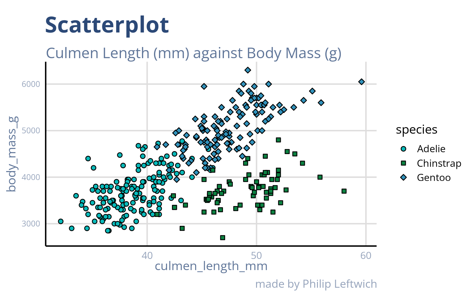
dodge <- 0.8

penguins |>
  drop_na(sex) |>
ggplot(    aes(x = species,
           y = body_mass_g,
           fill = sex))+
  geom_violin(position = position_dodge(width = dodge), alpha = .4)+
  geom_boxplot(position = position_dodge(width = dodge), width = .5, outliers = FALSE, show.legend = FALSE)+
  labs(title= "Boxplot",
       subtitle = "A comparison of Body Mass (g) by Sex and Species",
caption = "made by Philip Leftwich") 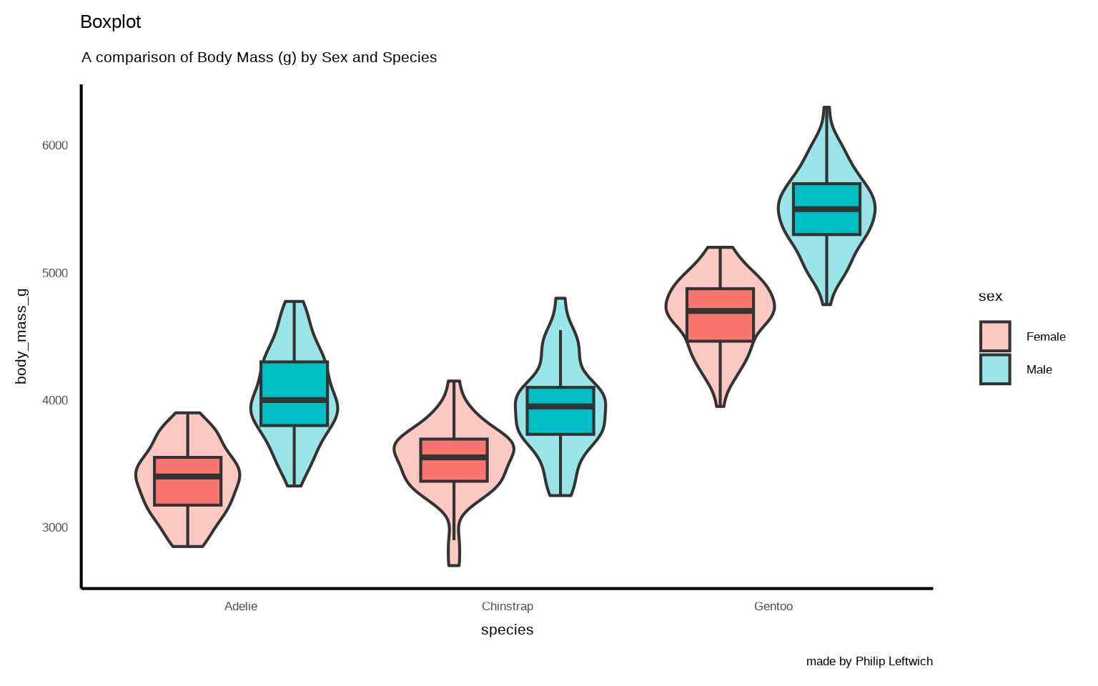
dodge <- 0.8

penguins |>
  drop_na(sex) |>
ggplot(    aes(x = species,
           y = body_mass_g,
           fill = sex))+
  geom_violin(position = position_dodge(width = dodge), alpha = .4)+
  geom_boxplot(position = position_dodge(width = dodge), width = .5, outliers = FALSE, show.legend = FALSE)+
  labs(title= "Boxplot",
       subtitle = "A comparison of Body Mass (g) by Sex and Species",
       caption = "made by Philip Leftwich") +
    theme_brand(axis_type  = "categorical")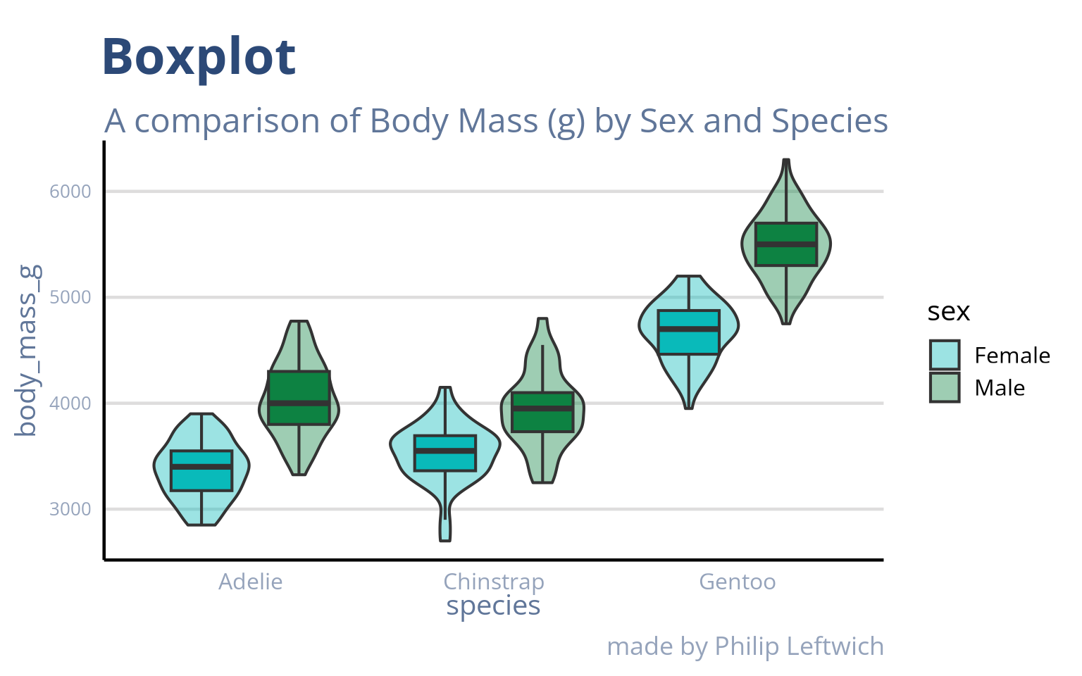
Task
This file when run now defines A named colour palette and a base theme function (theme_yourbrand)
Right now, your theme function is a standalone script — usable only within the current project. To ensure it can be shared, versioned, and applied consistently across analyses and colleagues, the correct next step is to encapsulate it in an R package